 “They used a Burr XII extreme value distribution?”
“Yeah, that’s what I’ve heard.”
“What the heck is that?”
“My best guess: it implies that Aaron Burr has bene cloned at least 11 times in secret laboratories.”
“Why would that have extreme value?”
“Suppose you wanted to stop the nefarious creators of 11 Alexander Hamilton clones….”
“I don’t think that theory deserves a very widespread distribution.”
But Seriously Folks
Several scholars, including one affiliated with the CME Group and one with Morgan Stanley, have together announced a new framework for quantifying the risk of an equity portfolio, a Bayesian framework that makes use of a Burr XII distribution.
As readers of AllAboutAlpha may recall, from here and here: though Thomas Bayes himself lived and died in the 18th century, the way of thinking about probability theory that has come to be associated with his name remains a very powerful force in today’s financial world.
The eight authors of the new study seek to add to “the existing literature of Bayesian VaR methods by … considering the … general class of Burr XII extreme value distributions “ and by estimating error bounds.
What does that mean?
Here’s a standard example of Bayesian methods: Suppose we know of a certain population (say, American women with an income above a certain level), that 90% of its members own automobiles. We also know that Alice Jones is a member of that population. Our first estimate, then, is that there is 90% likelihood that Jones owns an automobile. If we later seek to gather more facts and clarity on the subject, this 90% figure serves as what Bayesians call our “prior.”
Now: in this population (P), bike ownership is not very widespread, but we have the numbers for it. We will say that among those in P who own an automobile, 10% also own a bike. Among those in P who don’t own an automobile, 20% own a bike. These figures,[which we might also write if we please as .10 and .20] are “conditional” probabilities. We do some checking and learn something new about Jones. She owns a bike.
Can we now do anything to modify our initial .90 estimate? The ownership of bikes in this populatio ncorrelates positively, however loosely, with the non-ownership of cars, so the new datum should bring the probability somewhat lower than the prior. To be precise, the new (posterior) probability that Jones owns a car is 9/11, or roughly .82.
Path-Dependent Probability
Nobody argues with the math. But it has come to be associated with a controversial method and an interpretation of what probabilistic statements really mean. Bayesians take probability to be an expression of the level of confidence that a rational person will have in a certain fact or outcome given facts known to that rational person. This way of thinking makes statistical inference both more path-dependent and more subjective than some other views. You, the inquirer, should presumably as a rational person keep up-dating your view of the probability that Jones owns a car with every new relevant datum, with each posterior serving as the prior for the next link.
Ten years ago a paper by T.K. Siu and others proposed that a Bayesian approach to the implementation of Value at Risk “provides risk traders with the flexibility of adjusting their VaR models according to their subjective views.” The authors of that 2004 paper offered “an exact formula for the Bayesian VaR in the case of a single European call option.”
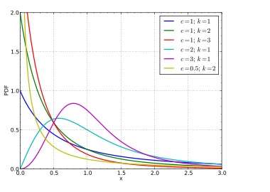
But our 2014 AUTHORS, Eric Hendries et al., propose to apply a similar approach to an equity portfolio with the assistance of Burr XII extreme value distributions. Despite my fantasy above, these are not clones. These are, rather, continuous frequency distributions of a type first discussed by Irving W. Burr in 1942. The Burr XII is often employed to model the distribution of income in a population, or to address the issue of flood frequency.
With these thoughts in mind, the authors approached four different hypothetical equity portfolios, such as a tech index basket portfolio. They tried to fit “a variety of heavy tailed and extreme value distributions to the data” and discovered “that the class of Burr distributions tended to fit the data better than the other classes of distribution we considered” and they selected this model to be incorporated into their subsequent Bayesian VaR model.
For more, continue here.


